Chapter 17
Factorial designs
Puzzle 1
Using Alice’s gene study data, compute Cohen’s d for the difference between self and other pictures in the C-gene condition, and then another Cohen’s d for the toggle switch condition? Use the pooled estimate for the standard deviation.
| Table 17.1 (reproduced): Alice's top secret research data | ||||
|---|---|---|---|---|
| C-gene | C-gene + toggle switch | |||
| Self | Other | Self | Other | |
| 43 | 9 | 75 | 80 | |
| 72 | 6 | 79 | 87 | |
| 44 | 6 | 87 | 88 | |
| 37 | 12 | 99 | 85 | |
| 61 | 9 | 85 | 93 | |
| 42 | 7 | 92 | 85 | |
| 59 | 12 | 87 | 86 | |
| 54 | 8 | 85 | 78 | |
| Mean | 51.50 | 8.62 | 86.12 | 85.25 |
| SD | 11.96 | 2.39 | 7.36 | 4.65 |
| Variance | 143.14 | 5.70 | 54.12 | 21.64 |
Let’s start with calculating Cohen’s d for the C-gene data. The ‘self’ and ‘other’ groups groups both contained 8 participants so the Ns will both be 8. The variances ($ s^2 $) for the resemblance scores in the self and other group are given in Table 17.1. Using these values we can obtain the pooled standard deviation
$$ \begin{aligned} s_p &= \sqrt{\frac{(N_S-1)s_S^2 + (N_O-1)s_O^2}{N_S + N_O -2}} \\ &= \sqrt{\frac{(8-1)143.14 + (8-1)5.70}{8 + 8 -2}} \\ &= \sqrt{\frac{1041.88}{14}} \\ &= \sqrt{74.42} \\ &= 8.63. \end{aligned} $$
We then use this pooled standard deviation to calculate d using the following equation:
$$ \begin{aligned} \hat{d} &= \frac{\bar{X}_S - \bar{X}_O}{s_p} \\ &= \frac{51.50-8.62}{8.63} \\ &= 4.97 \end{aligned} $$
So we end up with an effect size of $ = 4.97 $, which is frankly unrealistically large - you should be suspicious if you see a d this large in real research. In any case, resemblance scores in the self condition were 4.97 standard deviations higher than the other condition, suggesting that resemblance scores are extremely different in the same and other picture groups.
Moving onto when a toggle switch was also employed, the means and variances ($ s^2 $) for the resemblance scores in the self and other group are again in Table 17.1. Using these values we can obtain the pooled standard deviation
$$ \begin{aligned} s_p &= \sqrt{\frac{(N_S-1)s_S^2 + (N_O-1)s_O^2}{N_S + N_O -2}} \\ &= \sqrt{\frac{(8-1)54.12 + (8-1)21.64}{8 + 8 -2}} \\ &= \sqrt{\frac{530.32}{14}} \\ &= \sqrt{37.88} \\ &= 6.15. \end{aligned} $$
We then use this pooled standard deviation to calculate d using the following equation:
$$ \begin{aligned} \hat{d} &= \frac{\bar{X}_S - \bar{X}_O}{s_p} \\ &= \frac{86.12-85.25}{6.15} \\ &= 0.14 \end{aligned} $$
So we end up with an effect size of $ = 0.14 $. Resemblance scores in the self condition were 0.14 standard deviations higher than the other condition, which is a tiny effect, suggesting that resemblance scores are very similar in the same and other picture groups.
Puzzle 2
On Zach’s journey he discovered that people can perform better on a statistics test if they take the test under a fake name (Reality Check 8.1). He found some data in which 182 men and women took a statistics test. They were assigned to one of three groups: take the test using their own name, a fake female name or a fake male name. The outcome was the percentage on the test. Zach ran a factorial linear model (ANOVA) to see whether participant gender, the type of name they used, or the interaction between these variables affected test results. However, when the summary of results appeared on his diePad (Table 17.5), Milton used the magic eraser tool to delete some of the numbers. He’s an eisel like that. Help Zach to fill in the blanks and to determine whether each F is significant at p = 0.05. [Tip: think about the degrees of freedom for each predictor variable].
First we need to compute the degrees of freedom. For the variable Sex there were $ k = 2 $ groups, so we get $ df_S = k - 1 = 1 $, for the variable Name there were $ k = 3 $ groups, so we get $ df_N = k - 1 = 2 $, and for the interaction term we get $ df_{SN} = df_S df_N = 2 = 2$.
Now we have the $ df_{SN} $, we can work back from the mean squares for the interaction term to find the sum of squares
$$ \begin{aligned} MS_{S\times N} &= \frac{SS_{S\times N}}{df_{S\times N}} \\ SS_{S\times N} &= MS_{S\times N} \times df_{S\times N} \\ &= 1023.50 \times 2 \\ &= 2047. \end{aligned} $$
From $ SS_{SN} $ we can calculate the sum of squared errors for Sex, $ SS_{S} $, from the other values in the table
$$ \begin{aligned} SS_{M} &= SS_{S} + SS_{N} + SS_{S\times N} \\ SS_{S} &= SS_{M} - SS_{N} - SS_{S\times N}\\ &= 7854.25 - 351.50 - 2047 \times 2 \\ &= 5455.75. \end{aligned} $$
Using this value, we can work out the mean squared error for Sex, $ MS_S $, as
$$ \begin{aligned} MS_{S} &= \frac{SS_{S}}{df_S} \\ &= \frac{5455.75}{1}\\ &= 5455.75. \end{aligned} $$
We also now have enough information to work out the mean squared error for Name, $ MS_N $, as
$$ \begin{aligned} MS_{N} &= \frac{SS_{N}}{df_N} \\ &= \frac{351.50}{2}\\ &= 175.75. \end{aligned} $$
We also need the mean squared error for Residual, $ MS_R $, which we can get from the values in the table
$$ \begin{aligned} MS_{R} &= \frac{SS_{R}}{df_R} \\ &= \frac{69226.70}{176}\\ &= 393.33. \end{aligned} $$
All that remains is the three F-statistics, which we can get from this equation:
$$ F = \frac{MS_{\text{Effect}}}{MS_{\text{Residual}}} $$
For the variable Sex
$$ F_S = \frac{MS_{S}}{MS_{R}} = \frac{5455.75}{393.33} = 13.87. $$
For the variable Name
$$ F_N = \frac{MS_{N}}{MS_{R}} = \frac{175.75}{393.33} = 0.44. $$
For the Sex:Name interaction
$$ F_{S \times N} = \frac{MS_{S \times N}}{MS_{R}} = \frac{1023.50}{393.33} = 2.60. $$
The completed table looks like this
| Source | SS | df | MS | F |
|---|---|---|---|---|
| Model | 7854.25 | 5 | ||
| Sex | 5455.75 | 1 | 5455.75 | 13.87 |
| Name Type | 351.50 | 2 | 175.75 | 0.44 |
| Sex `\(\times\)` Name Type | 2047.00 | 2 | 1023.50 | 2.60 |
| Residual | 69226.70 | 176 | 393.33 |
With respect to significance, let’s assume $ = 0.05 $. The residual term has $ df_R = 176 $ and the tables in the book only go up to $ df_R = 100 $, so we’ll use this value (which will be quite conservative so if we find significance with this value we know that p < 0.05).
For the effect of Sex the critical value from the table in the book is $ F(1, 100) = 3.94 $. The observed F is greater than this value so the main effect of Sex was significant at p < 0.05. That is, accuracy scores were significantly different in men and women in this study.
For the effect of Name the critical value from the table in the book is $ F(2, 100) = 3.09 $. The observed F is less than this value so the main effect of Name was not significant at p < 0.05. That is, accuracy scores were not significantly different when people took the test under different names.
For the Sex:Name interaction the critical value from the table in the book is again $ F(2, 100) = 3.09 $. The observed F is less than this value so the interaction was not significant at p < 0.05. That is, the effect of sex on accuracy scores was not significantly moderated by whether people took the test under different names. Remember we have used conservative degrees of freedom here because we needed to use tabulated critical values.
Puzzle 3
Figure 17.10 shows the means for the interaction effect in Table 17.5. Interpret this effect.
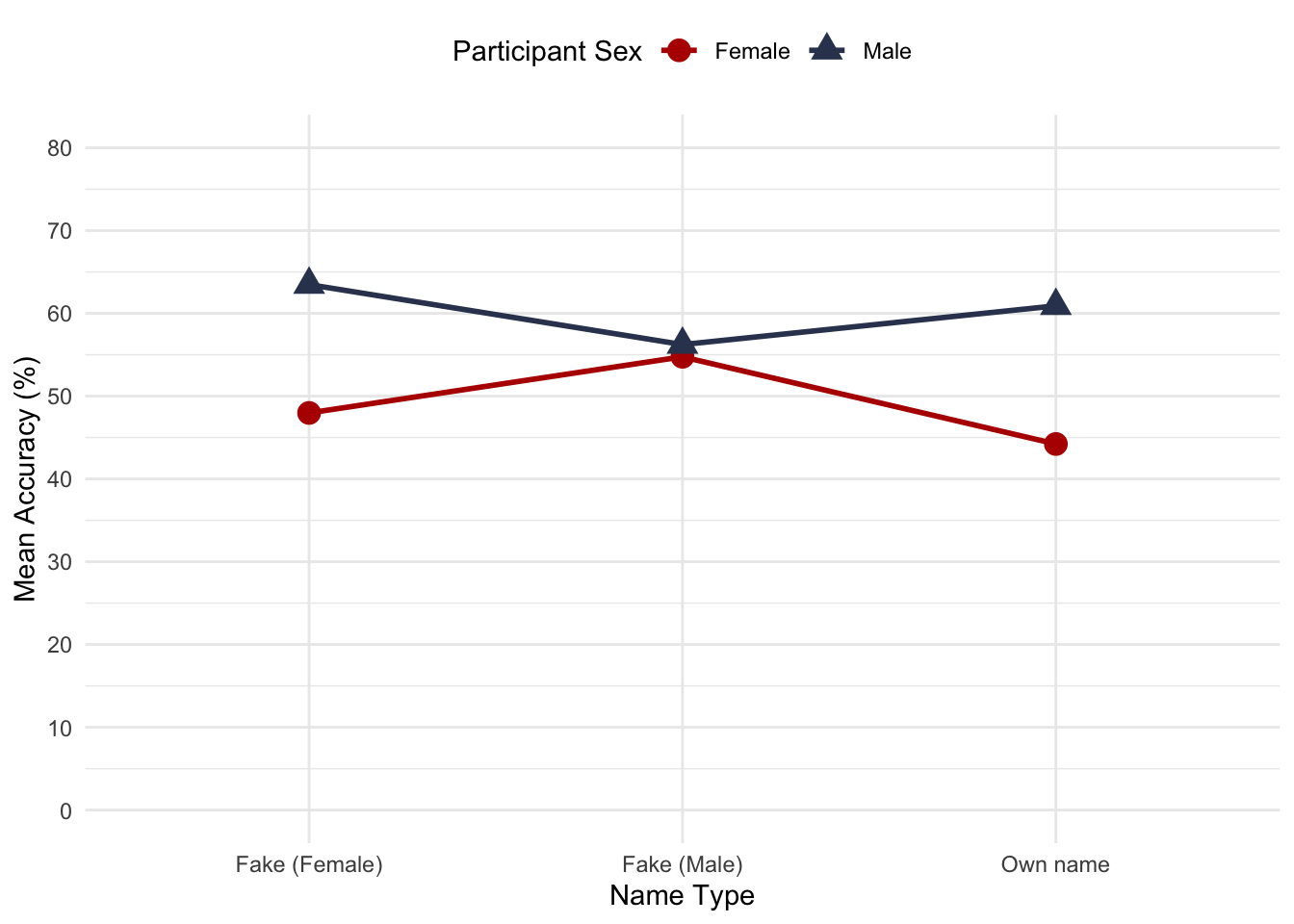
Figure 1: Figure 17.10 (reproduced)
When the test was completed using a fake female name or their own name, males outperformed females in this sample, but when the test was completed using a fake male name this differences was wiped out: males and females performed at the same level.
Puzzle 4
Alice tried to see whether she could use her toggle switch therapy to rehabilitate the zombie Code 1318 workers. She took 14 zombies, and 14 humans with facial injuries as controls. Half of each group received her original C-gene therapy, whereas the other half received a toggle switch as well. All participants were asked to study a picture of themselves before their injury/zombification. The outcome was how closely they resembled the photo as a percentage. The data are in Table 17.6. Fit a two-way linear model to these data to test the main effects of therapy (C-gene vs. C-gene + toggle switch), species (human vs. Zombie) and their interaction. Is each F-ratio significant?
| Table 17.6 (reproduced): Alice's zombie rehabilitation data | ||||
|---|---|---|---|---|
| C-gene | C-gene + toggle switch | |||
| Human | Zombie | Human | Zombie | |
| 75 | 48 | 89 | 53 | |
| 62 | 62 | 79 | 100 | |
| 56 | 63 | 75 | 60 | |
| 43 | 57 | 96 | 100 | |
| 34 | 48 | 85 | 63 | |
| 41 | 60 | 85 | 70 | |
| 55 | 59 | 78 | 74 | |
| Mean | 52.29 | 56.71 | 83.86 | 74.29 |
| SD | 14.02 | 6.26 | 7.22 | 18.82 |
| Variance | 196.57 | 39.24 | 52.14 | 354.24 |
Notes:
- Throughout, we will use means and variances from Table 17.6 (reproduced above).
- I will denote human as H, zombie as Z, c-gene as C and c-gene and toggle switch as T. For example, the group of humans who had the c-gene will be denoted as HC and the zombies who has c-gene and toggle switch as ZT.
The model sum of squares, SSM, is given by
$$ SS_M = \sum_{k = 1}^k n_k(\bar{x}_k-\bar{x}_g)^2, $$
in which $ n_k $ is the sample size of group k, $ {x}_k $ is the mean of group k, and $ {x}_g $ is the mean of all scores.
The mean of all scores is
$$ \bar{x}_g = \frac{\sum x_i}{N} = \frac{1870}{28} = 66.79. $$
We then need to apply
$$ n_k(\bar{x}_k-\bar{x}_g)^2 $$ to each group in turn
$$ \begin{aligned} HC &= 7(52.29-66.79)^2 = 1471.75 \\ ZC &= 7(56.71-66.79)^2 = 711.2448 \\ HT &= 7(83.86-66.79)^2 = 2039.694 \\ ZT &= 7(74.29-66.79)^2 = 393.75 \end{aligned} $$
We add these individual sums of squares to get SSM, as follows:
$$ \begin{aligned} SS_M &= 1471.75 + 711.2448 + 2039.694 + 393.75 \\ &= 4616.439. \end{aligned} $$
We have compared $ k = 4 $ groups so the associated degrees of freedom are $ df_M = k -1 = 3$.
The sum of squares for the effect of gene therapy, SSG, is given by the same equation but using means for all participants who underwent the different therapies (irrespective of whether they were zombies or humans).
$$ SS_G = \sum_{k = 1}^k n_k(\bar{x}_k-\bar{x}_g)^2, $$
The mean of all 14 c-gene resemblance scores is
$$ \bar{x}_C = \frac{\sum x_i}{N} = \frac{763}{14} = 54.50. $$
The mean of all 14 c-gene and toggle switch resemblance scores is
$$ \bar{x}_T = \frac{\sum x_i}{N} = \frac{1107}{14} = 79.07. $$
Therefore, the SS in each group is
$$ SS_C = n_C(\bar{x}_C-\bar{x}_g)^2 = 14(54.5-66.79)^2 = 2114.617 $$
and
$$ SS_T = n_T(\bar{x}_T-\bar{x}_g)^2 = 14(79.07-66.79)^2 = 2111.178 $$
To get SSG we add these group sums of squares
$$ \begin{aligned} SS_G &= SS_C + SS_T \\ &= 2114.617 + 2111.178 \\ &= 4225.795. \end{aligned} $$
We have compared $ k = 2 $ groups of data so the associated degrees of freedom are $ df_G = k - 1 = 1$, and the associated mean squared error is
$$ MS_G = \frac{SS_G}{df_G} = \frac{4225.795}{1} = 4225.795. $$
The sum of squares for the effect of species, SSS, is given by the same equation but using means for all humans and zombies (irrespective of the type of therapy they underwent).
$$ SS_S = \sum_{k = 1}^k n_k(\bar{x}_k-\bar{x}_g)^2, $$
The mean of all 14 human scores is
$$ \bar{x}_H = \frac{\sum x_i}{N} = \frac{953}{14} = 68.07. $$
The mean of all 14 zombie resemblance scores is
$$ \bar{x}_Z = \frac{\sum x_i}{N} = \frac{917}{14} = 65.50. $$
Therefore, the SS in each group is, for humans
$$ SS_H = n_H(\bar{x}_H-\bar{x}_g)^2 = 14(68.07-66.79)^2 = 22.9376 $$ and zombies
$$ SS_Z = n_Z(\bar{x}_Z-\bar{x}_g)^2 = 14(65.50-66.79)^2 = 23.2974 $$
To obtain SSS we add the SS for the human and zombie groups
$$ \begin{aligned} SS_S &= SS_H + SS_Z \\ &= 22.9376 + 23.2974 \\ &= 46.235. \end{aligned} $$
We have compared $ k = 2 $ groups of data so the associated degrees of freedom are $ df_S = k - 1 = 1$, and the associated mean squared error is
$$ MS_S = \frac{SS_S}{df_S} = \frac{46.235}{1} = 46.235. $$
The sum of squares for the interaction effect of gene therapy and species, $ SS_{G S} $, is given by
$$ \begin{aligned} SS_{G \times S} &= SS_M - SS_G - SS_S \\ &= 4616.439 - 4225.795 - 46.235 \\ &= 344.409. \end{aligned} $$
The associated degrees of freedom are $ df_{G S} = df_M - df_S - df_G = 3 - 1 - 1 = 1$, and the associated mean squared error is
$$ MS_{G \times S} = \frac{SS_{G \times S}}{df_{G \times S}} = \frac{344.409}{1} = 344.409. $$
The residual sum of squares SSR is given by
$$ SS_R = \sum (Y_{ik} - \bar{Y}_{k})^2, $$
which basically means that within each group we calculate the difference between each score and the group mean, square these differences and sum them. The associated degrees of freedom for each group are $ n - 1 $, which is 6 in each case (because there are $ n = 7 $ scores per group). This table shows the process
| Calculating sums of squares within each group | ||||
|---|---|---|---|---|
| Resemblance $x_{ij}$ |
Mean $\bar{x}_k$ |
Deviation $x_{ij}-\bar{x}_k$ |
Deviation squared $(x_{ij}-\bar{x}_k)^2$ |
|
| Zombie - C-Gene | ||||
| 1 | 48 | 56.71 | -8.71 | 75.8641 |
| 2 | 62 | 56.71 | 5.29 | 27.9841 |
| 3 | 63 | 56.71 | 6.29 | 39.5641 |
| 4 | 57 | 56.71 | 0.29 | 0.0841 |
| 5 | 48 | 56.71 | -8.71 | 75.8641 |
| 6 | 60 | 56.71 | 3.29 | 10.8241 |
| 7 | 59 | 56.71 | 2.29 | 5.2441 |
| SS | 235.429 | |||
| df | 6.000 | |||
| Zombie - C-Gene + Toggle Switch | ||||
| 8 | 53 | 74.29 | -21.29 | 453.2641 |
| 9 | 100 | 74.29 | 25.71 | 661.0041 |
| 10 | 60 | 74.29 | -14.29 | 204.2041 |
| 11 | 100 | 74.29 | 25.71 | 661.0041 |
| 12 | 63 | 74.29 | -11.29 | 127.4641 |
| 13 | 70 | 74.29 | -4.29 | 18.4041 |
| 14 | 74 | 74.29 | -0.29 | 0.0841 |
| SS | 2,125.429 | |||
| df | 6.000 | |||
| Human - C-Gene | ||||
| 15 | 75 | 52.29 | 22.71 | 515.7441 |
| 16 | 62 | 52.29 | 9.71 | 94.2841 |
| 17 | 56 | 52.29 | 3.71 | 13.7641 |
| 18 | 43 | 52.29 | -9.29 | 86.3041 |
| 19 | 34 | 52.29 | -18.29 | 334.5241 |
| 20 | 41 | 52.29 | -11.29 | 127.4641 |
| 21 | 55 | 52.29 | 2.71 | 7.3441 |
| SS | 1,179.429 | |||
| df | 6.000 | |||
| Human - C-Gene + Toggle Switch | ||||
| 22 | 89 | 83.86 | 5.14 | 26.4196 |
| 23 | 79 | 83.86 | -4.86 | 23.6196 |
| 24 | 75 | 83.86 | -8.86 | 78.4996 |
| 25 | 96 | 83.86 | 12.14 | 147.3796 |
| 26 | 85 | 83.86 | 1.14 | 1.2996 |
| 27 | 85 | 83.86 | 1.14 | 1.2996 |
| 28 | 78 | 83.86 | -5.86 | 34.3396 |
| SS | 312.857 | |||
| df | 6.000 | |||
We obtain SSR by adding the sums of squares for each group (in the table)
$$ \begin{aligned} SS_R &= SS_{ZC} + SS_{ZT} + SS_{HC} + SS_{HT} \\ &= 235.429 + 2125.429 + 1179.429 + 312.857 \\ &= 3853.144. \end{aligned} $$
The associated degrees of freedom are
$$ \begin{aligned} df_R &= df_{ZC} + df_{ZT} + df_{HC} + df_{HT} \\ &= 6 + 6 + 6 + 6 \\ &= 24. \end{aligned} $$
The resulting mean squares is
$$ MS_R = \frac{SS_R}{df_R} = \frac{3853.144}{24} = 160.548 $$
All that remains is the three F-statistics, which we can get from this equation:
$$ F = \frac{MS_{\text{Effect}}}{MS_{\text{Residual}}} $$
For the variable Therapy
$$ F_G = \frac{MS_G}{MS_R} = \frac{4225.795}{160.548} = 26.32. $$
For the variable Species
$$ F_S = \frac{MS_S}{MS_R} = \frac{46.235}{160.548} = 0.29. $$
For the Sex:Name interaction
$$ F_{G \times S} = \frac{MS_{G \times S}}{MS_R} = \frac{344.409}{160.548} = 2.14. $$
The completed table looks like this (This table was generated using R, which retains all decimal places, so there are differences in the SS in the table to those we computed due to the rounding we used in the hand calculations, but note that the Fs are the same as our hand calculations.)
| Source | SS | df | `\(F\)` | `\(p\)` |
|---|---|---|---|---|
| (Intercept) | 124889.29 | 1 | 777.90 | 0.00 |
| Species | 46.29 | 1 | 0.29 | 0.60 |
| Therapy | 4226.29 | 1 | 26.32 | 0.00 |
| Species:Therapy | 343.00 | 1 | 2.14 | 0.16 |
| Residuals | 3853.14 | 24 |
With respect to significance, let’s assume $ = 0.05 $. The residual term has $ df_R = 24 $ and each effect has a 1 degree of freedom so the critical value from the table in the book is $ F(1, 24) = 4.26 $.
For the effect of Species the observed $ F = 0.29 $ is smaller than the critical value of 4.26 so the main effect of Species was not significant at p = 0.05. That is, resemblance scores were not significantly different in humans and zombies. From the table, the exact P = 0.60.
For the effect of Therapy the observed $ F = 26.32 $ is greater than the critical value of 4.26. The main effect of Therapy was significant at p < 0.05. That is, resemblance scores were significantly higher (we can tell this from the means) when the toggle switch was used than when it wasn’t. From the table, the exact P < 0.001.
For the Species:Therapy interaction the observed $ F = 2.14 $ is smaller than the critical value of 4.26 so the interaction between Species and Therapy was not significant at p = 0.05. That is, the effect of therapy on resemblance scores was not significantly moderated by whether people were humans or zombies. From the table, the exact P = 0.16.
Puzzle 5
Draw the interaction graph for Alice’s zombie rehabilitation data (Table 17.5) and interpret the interaction effect.
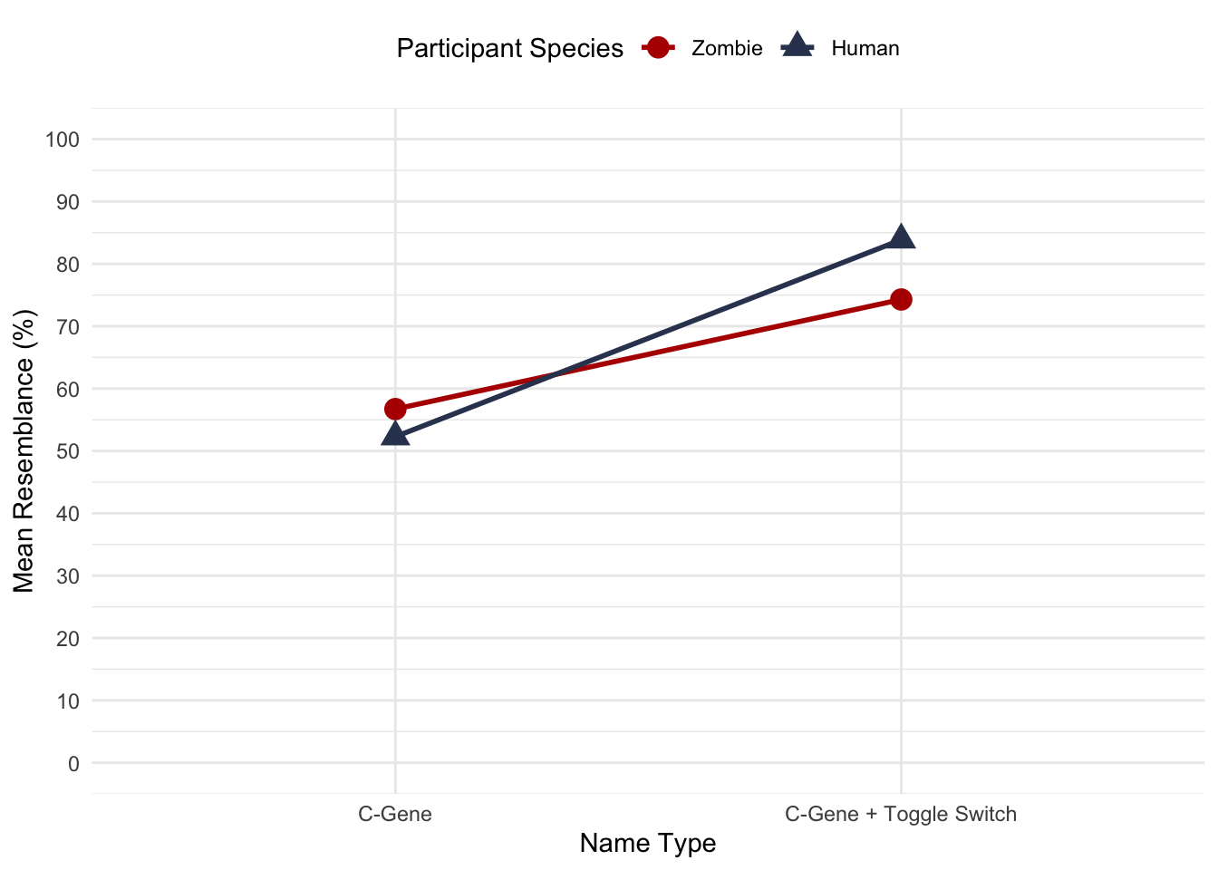
Figure 2: Interaction plot for the rehabilitation data
It looks as though after c-gene therapy resemblance scores were very similar for humans and zombies, but after the c-gene and toggle switch therapy resemblance scores were higher in general (than for c-gene therapy alone) but especially so for humans. From Puzzle 5 we know that the interaction effect was not significant suggesting that the differences between humans and zombies in each therapy group are statistically comparable.
Puzzle 6
Output 17.8 to Output 17.10 show the Bayes factors for each effect in Alice’s zombie rehabilitation data. Interpret each Bayes factor: do they support or contradict the findings from the linear model?
The main effect of gene Therapy has a Bayes factor of 647.73 (Output 17.8), suggesting that we should shift our belief in the alternative hypothesis relative to the null by a factor of about 650. This is substantial evidence that therapy had an effect on resemblance scores.
When we add the main effect of Species and see how it improves the model compared to when we only include gene therapy as a predictor (Output 17.9), the Bayes factor is 0.37. This value is less than 1 suggesting we shift our belief towards the null. In short there is evidence for the null.
Finally, when we include the interaction effect and compare this to the model that included the main effects (Output 17.10), the Bayes factor for the interaction term is 0.86. Again, this value is less than 1 suggesting we shift our belief towards the null. However, the value is quite close to 1 suggesting quite weak evidence for the null (our beliefs shouldn’t shift too much towards the null).
These results are consistent with the linear model in that there was strong evidence for an overall effect of the therapy on resemblance scores, and there was also support for the idea that this is not moderated by the species undergoing treatment.
Bayes factor analysis
--------------
[1] Therapy : 647.7348 ±0%

Against denominator:
  Intercept only
---
Bayes factor type: BFlinearModel, JZS
Output 17.8: Testing the main effect of therapy with a Bayes factor using lmBF() in R
Bayes factor analysis
--------------
[1] Therapy + Species : 0.376888 ±1.22%

Against denominator:
  Resemblance ~ Therapy
---
Bayes factor type: BFlinearModel, JZS
Output 17.9: Testing the main effect of species with a Bayes factor using lmBF() in R
Bayes factor analysis
--------------
[1] Therapy + Species + Therapy:Species : 0.858355 ±2.83%

Against denominator:
  Resemblance ~ Therapy + Species
---
Bayes factor type: BFlinearModel, JZS
Output 17.10: Testing the interaction effect with a Bayes factor using lmBF() in R
Puzzle 7
Milton and Roediger were having an argument about whether cats or dogs were the most gullible. Milton cited a study in which dogs were given the choice of either a large or small quantity of food on 12 occasions. On 6 of these, the dog chose one or other quantities without interference. On the other 6 occasions, their owner used ostensive cues to mislead the dog into choosing the smaller portion: the owner picked up the bowl, put it to their mouth, looked at the food, then the dog and then said ‘Ow wow, this is good, this is so good’. Without influence the dogs chose the larger portion more than when the owner had used ostensive cues to make the smaller portion seem better. Milton argued that this proved that dogs were stupid. To counter this, Roediger organized a replication study in which cats were tested too. Table 17.7 shows the number of trials (out of 6) that 12 dogs and 12 cats chose the larger portion of food when left to their own devices (no influence) and when their owner tried to mislead them using ostensive cues. Compute the two-way linear model for these data to test the main effects of influence (none vs. misleading), species (cat vs. dog) and their interaction. Is each F-ratio significant?
| Table 17.7 (reproduced): Data on animal food choices after human influence (or not) | ||||
|---|---|---|---|---|
| No influence | Counterproductive influence | |||
| Dog | Cat | Dog | Cat | |
| 4 | 6 | 4 | 4 | |
| 5 | 4 | 3 | 4 | |
| 5 | 5 | 2 | 5 | |
| 5 | 4 | 2 | 4 | |
| 5 | 5 | 2 | 4 | |
| 5 | 4 | 3 | 5 | |
| Mean | 4.833 | 4.667 | 2.667 | 4.333 |
| SD | 0.408 | 0.816 | 0.816 | 0.516 |
| Variance | 0.167 | 0.667 | 0.667 | 0.267 |
Notes:
- Throughout, we will use means and variances from Table 17.7 (reproduced above).
- I will denote dog as D, cat as C, no influence as N and counter-productive influence as I. For example, the group of cats who had counter-productive influence will be denoted as IC and the dogs who had no influence as ND.
The model sum of squares, SSM, is given by
$$ SS_M = \sum_{k = 1}^k n_k(\bar{x}_k-\bar{x}_g)^2, $$
in which $ n_k $ is the sample size of group k, $ {x}_k $ is the mean of group k, and $ {x}_g $ is the mean of all scores.
The mean of all scores is
$$ \bar{x}_g = \frac{\sum x_i}{N} = \frac{99}{24} = 4.125. $$
We then need to apply
$$ n_k(\bar{x}_k-\bar{x}_g)^2 $$
to each group in turn
$$ \begin{aligned} ND &= 6(4.833-4.125)^2 = 3.008 \\ NC &= 6(4.667-4.125)^2 = 1.763 \\ ID &= 6(2.667-4.125)^2 = 12.755 \\ IC &= 6(4.333-4.125)^2 = 0.260 \end{aligned} $$
We add these individual sums of squares to get SSM, as follows:
$$ \begin{aligned} SS_M &= 3.008 + 1.763 + 12.755 + 0.260 \\ &= 17.786. \end{aligned} $$
We have compared $ k = 4 $ groups so the associated degrees of freedom are $ df_M = k -1 = 3$.
The sum of squares for the effect of human influence, SSH, is given by the same equation but using means for all participants who underwent the different type of influence (irrespective of whether they were dogs or cats).
$$ SS_H = \sum_{k = 1}^k n_k(\bar{x}_k-\bar{x}_g)^2, $$
The mean of all 12 scores from animals who experienced no influence is
$$ \bar{x}_N = \frac{\sum x_i}{N} = \frac{57}{12} = 4.75. $$
The mean of all 2 scores from animals who experienced counter-productive influence is
$$ \bar{x}_I = \frac{\sum x_i}{N} = \frac{42}{12} = 3.50. $$
Therefore, the SS in each group is
$$ SS_N = n_{N}(\bar{x}_{N}-\bar{x}_g)^2 = 12(4.75-4.125)^2 = 4.688 $$
and
$$ SS_I = n_I(\bar{x}_I-\bar{x}_g)^2 = 12(3.50-4.125)^2 = 4.687 $$
To get SSH we add these group sums of squares
$$ \begin{aligned} SS_H &= SS_N + SS_I \\ &= 4.687 + 4.687 \\ &= 9.374. \end{aligned} $$
We have compared $ k = 2 $ groups of data so the associated degrees of freedom are $ df_H = k - 1 = 1$, and the associated mean squared error is
$$ MS_H = \frac{SS_H}{df_H} = \frac{9.374}{1} = 9.374. $$
The sum of squares for the effect of species, SSS, is given by the same equation but using means for all humans and zombies (irrespective of the type of therapy they underwent).
$$ SS_S = \sum_{k = 1}^k n_k(\bar{x}_k-\bar{x}_g)^2, $$
The mean of all 12 dog scores is
$$ \bar{x}_D = \frac{\sum x_i}{N} = \frac{45}{12} = 3.75. $$
The mean of all 12 cat scores is
$$ \bar{x}_C = \frac{\sum x_i}{N} = \frac{54}{12} = 4.50. $$
Therefore, the SS in each group is, for dogs
$$ SS_D = n_D(\bar{x}_D-\bar{x}_g)^2 = 12(3.75-4.125)^2 = 1.688 $$ and cats
$$ SS_C = n_C(\bar{x}_C-\bar{x}_g)^2 = 12(4.50-4.125)^2 = 1.688 $$
To obtain SSS we add the SS for the cat and dog groups
$$ \begin{aligned} SS_S &= SS_D + SS_C \\ &= 1.688 + 1.688 \\ &= 3.376. \end{aligned} $$
We have compared $ k = 2 $ groups of data so the associated degrees of freedom are $ df_S = k - 1 = 1$, and the associated mean squared error is
$$ MS_S = \frac{SS_S}{df_S} = \frac{3.376}{1} = 3.376. $$
The sum of squares for the interaction effect of gene therapy and species, $ SS_{H S} $, is given by
$$ \begin{aligned} SS_{H \times S} &= SS_M - SS_H - SS_S \\ &= 17.786 - 9.374 - 3.376 \\ &= 5.036. \end{aligned} $$
The associated degrees of freedom are $ df_M - df_S - df_H = 3 - 1 - 1 = 1$, and the associated mean squared error is
$$ MS_{H \times S} = \frac{SS_{H \times S}}{df_{H \times S}} = \frac{5.036}{1} = 5.036. $$
The residual sum of squares SSR is given by
$$ SS_R = \sum (Y_{ik} - \bar{Y}_{k})^2, $$
which basically means that within each group we calculate the difference between each score and the group mean, square these differences and sum them. The associated degrees of freedom for each group are $ n - 1 $, which is 5 in each case (because there are $ n = 6 $ scores per group). This table shows the process
| Calculating sums of squares within each group | ||||
|---|---|---|---|---|
| Larger portion $x_{ij}$ |
Mean $\bar{x}_k$ |
Deviation $x_{ij}-\bar{x}_k$ |
Deviation squared $(x_{ij}-\bar{x}_k)^2$ |
|
| Dog - No Influence | ||||
| 1 | 4 | 4.833 | -0.833 | 0.693889 |
| 2 | 5 | 4.833 | 0.167 | 0.027889 |
| 3 | 5 | 4.833 | 0.167 | 0.027889 |
| 4 | 5 | 4.833 | 0.167 | 0.027889 |
| 5 | 5 | 4.833 | 0.167 | 0.027889 |
| 6 | 5 | 4.833 | 0.167 | 0.027889 |
| SS | 0.833 | |||
| df | 5.000 | |||
| Dog - Counterproductive Influence | ||||
| 7 | 4 | 2.667 | 1.333 | 1.776889 |
| 8 | 3 | 2.667 | 0.333 | 0.110889 |
| 9 | 2 | 2.667 | -0.667 | 0.444889 |
| 10 | 2 | 2.667 | -0.667 | 0.444889 |
| 11 | 2 | 2.667 | -0.667 | 0.444889 |
| 12 | 3 | 2.667 | 0.333 | 0.110889 |
| SS | 3.333 | |||
| df | 5.000 | |||
| Cat - No Influence | ||||
| 13 | 6 | 4.667 | 1.333 | 1.776889 |
| 14 | 4 | 4.667 | -0.667 | 0.444889 |
| 15 | 5 | 4.667 | 0.333 | 0.110889 |
| 16 | 4 | 4.667 | -0.667 | 0.444889 |
| 17 | 5 | 4.667 | 0.333 | 0.110889 |
| 18 | 4 | 4.667 | -0.667 | 0.444889 |
| SS | 3.333 | |||
| df | 5.000 | |||
| Cat - Counterproductive Influence | ||||
| 19 | 4 | 4.333 | -0.333 | 0.110889 |
| 20 | 4 | 4.333 | -0.333 | 0.110889 |
| 21 | 5 | 4.333 | 0.667 | 0.444889 |
| 22 | 4 | 4.333 | -0.333 | 0.110889 |
| 23 | 4 | 4.333 | -0.333 | 0.110889 |
| 24 | 5 | 4.333 | 0.667 | 0.444889 |
| SS | 1.333 | |||
| df | 5.000 | |||
We obtain SSR by adding the sums of squares for each group (in the table)
$$ \begin{aligned} SS_R &= SS_{ND} + SS_{NC} + SS_{ID} + SS_{IC} \\ &= 0.833 + 3.333 + 3.333 + 1.333 \\ &= 8.832. \end{aligned} $$
The associated degrees of freedom are
$$ \begin{aligned} df_R &= df_{ND} + df_{NC} + df_{ID} + df_{IC} \\ &= 5 + 5 + 5 + 5 \\ &= 20 \end{aligned} $$
The resulting mean squares is
$$ MS_R = \frac{SS_R}{df_R} = \frac{8.832}{20} = 0.442. $$
All that remains is the three F-statistics, which we can get from this equation:
$$ F = \frac{MS_{\text{Effect}}}{MS_{\text{Residual}}} $$
For the variable human Influence
$$ F_H = \frac{MS_H}{MS_R} = \frac{9.374}{0.442} = 21.21. $$
For the variable Species
$$ F_S = \frac{MS_S}{MS_R} = \frac{3.376}{0.442} = 7.64. $$
For the Influence:Species interaction
$$ F_{H \times S} = \frac{MS_{H \times S}}{MS_R} = \frac{5.036}{0.442} = 11.39. $$
The completed table looks like this (This table was generated using R, which retains all decimal places, so there are differences in some of the decimal places to those we computed by hand due to the rounding we used in the hand calculations.)
| Source | SS | df | `\(F\)` | `\(p\)` |
|---|---|---|---|---|
| (Intercept) | 408.37 | 1 | 924.62 | 0.00 |
| Species | 3.37 | 1 | 7.64 | 0.01 |
| Influence | 9.37 | 1 | 21.23 | 0.00 |
| Species:Influence | 5.04 | 1 | 11.42 | 0.00 |
| Residuals | 8.83 | 20 |
With respect to significance, let’s assume $ = 0.05 $. The residual term has $ df_R = 20 $ and each effect has a 1 degree of freedom so the critical value from the table in the book is $ F(1, 20) = 4.35 $.
For the effect of Species the observed $ F = 7.64 $ is greater than the critical value of 4.35. The main effect of Species was significant at p < 0.05. That is, the number of times the larger portion of food was chosen was significantly higher (we can tell this from the means) for cats compared to dogs. From the table, the exact P = 0.01
For the effect of Influence the observed $ F = 21.23 $ is greater than the critical value of 4.35. The main effect of Influence was significant at p < 0.05. That is, the number of times the larger portion of food was chosen was significantly higher (we can tell this from the means) when there was no human influence than when humans used counter-productive influence. From the table, the exact P < 0.001.
For the Species:Therapy interaction the observed $ F = 11.42 $ is greater than the critical value of 4.35. One interpretation of this effect is that the effect of the type of Influence used was significantly different in dogs and cats. We’ll interpret this effect further in the next puzzle. From the table, the exact P < 0.001.
Puzzle 8
Draw and interpret the interaction graph for Roediger’s food choice data (Table 17.7) and interpret the interaction effect.
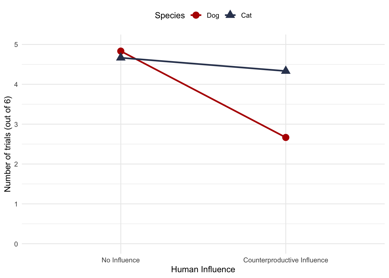
Figure 3: Interaction plot for the rehabilitation data
In Puzzle 7 we saw that the interaction effect was significant. This plot helps us to interpret this effect. We can interpret it in two equally-valid ways.
Interpretation 1: By focussing on the effect of species (i.e. the gaps between the circles and triangles) the plot shows that in the no influence condition, there was very little effect of species: cats and dogs chose the large portion of food on about the same number of trials on average. Conversely, when counter-productive influence was used dogs chose the larger portion fewer times than cats, on average. In other words, the effect of species seems to be moderated by the type of influence used.
Interpretation 2: By focussing on the effect of influence (i.e. the slopes of the lines) the plot shows that for cats, there was very little effect of influence: cats chose the large portion of food on about the same number of trials on average regardless of whether or not counter-productive influence was used. Conversely, for dogs, there was a larger effect (than for cats) of influence: they chose the larger portion fewer times, on average, when counter-productive influence was used than when it wasn’t. In other words, the effect of influence seems to be moderated by the species.
In a general sense, Milton’s conclusion that ‘dogs are stupid’ (or at least more so than cats) is supported by these data, which is unfortunate for Roediger.
Puzzle 9
Output 17.11 to Output 17.13 show the Bayes factors for each effect in Roediger’s animal influence data. Interpret each Bayes factor: do they support or contradict the findings from the linear model?
The main effect of human Influence has a Bayes factor of 16.09 (Output 17.11), suggesting that we should shift our belief in the alternative hypothesis relative to the null by a factor of about 16. This is substantial evidence that the type of influence had an effect on how many times the larger food portion was selected.
When we add the main effect of Species and see how it improves the model compared to when we only include human influence as a predictor (Output 17.12), the Bayes factor is about 2. This value suggests we shift our belief away from the null by a factor of 2. In short there is some evidence that the type of species had an effect on how many times the larger food portion was selected.
Finally, when we include the interaction effect and compare this to the model that included the main effects (Output 17.13), the Bayes factor for the interaction term is 9.58. This is substantial evidence that the effect of the type of influence on how many times the larger food portion was selected was moderated by the species.
These results are consistent with the linear model in that there was strong evidence for an overall effect of the influence method and it’s interaction with species. One slight difference is the Bayes factors probably show weaker support for the main effect of species than the linear model, although this effect isn’t of specific interest given the interaction term.
Bayes factor analysis
--------------
[1] Influence : 16.0891 ±0%

Against denominator:
  Intercept only
---
Bayes factor type: BFlinearModel, JZS
Output 17.11: Testing the main effect of influence with a Bayes factor using lmBF() in R
Bayes factor analysis
--------------
[1] Influence + Species : 1.99659 ±1.63%

Against denominator:
  FoodChoice ~ Influence
---
Bayes factor type: BFlinearModel, JZS
Output 17.12: Testing the main effect of species with a Bayes factor using lmBF() in R
Bayes factor analysis
--------------
[1] Influence + Species + Influence:Species : 9.584772 ±2.71%

Against denominator:
  FoodChoice ~ Influence + Species
---
Bayes factor type: BFlinearModel, JZS
Output 17.13: Testing the interaction effect with a Bayes factor using lmBF() in R
Puzzle 10.
Output 17.14 shows a robust analysis of Roediger’s animal influence data (Table 17.7). Interpret the output: do any of your conclusions change from when you fitted the normal linear model?
The main effect of human Influence is very significant using a robust test (p = 0.0001), suggesting that the type of influence had an effect on how many times the larger food portion was selected. This result is consistent with the linear model.
The main effect of Species is non-significant using a robust test (p = 0.063), which conflicts with the findings of the linear model. However, this effect isn’t of specific interest given the interaction term.
Finally, the interaction effect is very significant using a robust test (p = 0.0003) suggesting that the species moderated the effect that the type of influence had on how many times the larger food portion was selected.
$Qa (Species)
[1] 4.326923

$A.p.value
[1] 0.063

$Qb (Influence)
[1] 20.94231

$B.p.value
[1] 0.001

$Qab (Interaction)
[1] 14.01923

$AB.p.value
[1] 0.003

$means
     [,1] [,2]
[1,] 4.25  4.5
[2,] 2.50  5.0
Output 17.14: Robust analysis of Roediger’s animal influence data