Chapter 14
The General Linear Model
Puzzle 1
In Chapter 13, we looked at an example of how big a correlation there was between openness to new relationships (Alternatives) and the extent to which your partner matched your ideal (Ideal). The data are in Table 13.4 (in the book and reproduced below). Calculate the parameters of the linear model for openness to new relationships being predicted from how closely a partner matches the person’s ideal.
| Table 13.4 (reproduced): Data on neuroticism and relationship commitment based on Kurdek (1997) | |||||
|---|---|---|---|---|---|
| Neuroticism | Rewards | Costs | Ideal | Alternatives | |
| 1 | 28 | 4 | 2 | 4 | 4 |
| 2 | 22 | 5 | 3 | 4 | 1 |
| 3 | 31 | 5 | 3 | 5 | 2 |
| 4 | 49 | 3 | 4 | 1 | 3 |
| 5 | 15 | 5 | 1 | 4 | 2 |
| 6 | 53 | 1 | 2 | 3 | 5 |
| 7 | 43 | 2 | 4 | 2 | 5 |
| 8 | 30 | 4 | 2 | 4 | 3 |
| 9 | 15 | 4 | 1 | 4 | 1 |
| 10 | 18 | 3 | 1 | 3 | 3 |
| Mean | 30.40 | 3.60 | 2.30 | 3.40 | 2.90 |
| SD | 13.83 | 1.35 | 1.16 | 1.17 | 1.45 |
Openness to new relationships is represented by the variable Alternatives, and we want to predict this variable from Ideal, which is how closely a partner matches the person’s ideal. The model can be expressed as follows:
$$ \begin{aligned} Y_i &= b_0 + b_1X_i + \epsilon_i \\ \text{Alternatives}_i &= b_0 + b_1\text{Ideal}_i + \epsilon_i \end{aligned} $$
The parameters mentioned in the puzzle allude to the two values of b. This puzzle is, therefore, asking us to calculate estimates for $ b_0 $ and $ b_1 $ in the model. The first step is to calculate the squared deviations for the predictor variable (Ideal), and the cross-product deviations, which are shown in the following table.
| Calculating the sum of squared deviations for $x$ ($SS_x$) and the sum of cross-product deviations ($SCP$) between $x$ and $y$ | ||||||
|---|---|---|---|---|---|---|
| Alternatives $(y_i)$ |
Ideal $(x_i)$ |
$(x_i-\bar{x})$ | $(x_i-\bar{x})^2$ | $(y_i-\bar{y})$ | $(x_i-\bar{x})(y_i-\bar{y})$ | |
| 4 | 4 | 0.6 | 0.36 | 1.1 | 0.66 | |
| 1 | 4 | 0.6 | 0.36 | -1.9 | -1.14 | |
| 2 | 5 | 1.6 | 2.56 | -0.9 | -1.44 | |
| 3 | 1 | -2.4 | 5.76 | 0.1 | -0.24 | |
| 2 | 4 | 0.6 | 0.36 | -0.9 | -0.54 | |
| 5 | 3 | -0.4 | 0.16 | 2.1 | -0.84 | |
| 5 | 2 | -1.4 | 1.96 | 2.1 | -2.94 | |
| 3 | 4 | 0.6 | 0.36 | 0.1 | 0.06 | |
| 1 | 4 | 0.6 | 0.36 | -1.9 | -1.14 | |
| 3 | 3 | -0.4 | 0.16 | 0.1 | -0.04 | |
| Mean | 2.90 | 3.40 | ||||
| Sum | 12.40 | −7.60 | ||||
We add the squared deviations to get the value of 12.4 shown at the bottom of column 5, and we also add the cross-product deviations to get the value of $ -7.6 $ shown at the bottom of the final column.
To calculate an estimate of $ b_1 $ we divide the sum of cross-product deviations by the sum of squared deviations for the predictor
$$ \hat{b}_1 = \frac{SCP}{SS_x} = \frac{-7.6}{12.4} = -0.61 $$
Now, on to the constant, $ b_0 $; this value tells us about the overall level of the outcome variable. I have put hats on the bs to remind you that these are estimated values. If we want to make the constant, $ b_0 $, the subject of the equation that defines the model we rearrange it:
$$ \begin{aligned} \hat{Y}_i &= \hat{b}_0 + \hat{b}_1X_i \\ \hat{b}_0 &= \hat{Y}_i-\hat{b}_1X_i \end{aligned} $$
If we replace the X and Y with the symbols for their respective means, and plug the values of those means in (see Table 1) we can estimate the constant, $ b_0 $:
$$ \begin{aligned} \hat{b}_0 &= \hat{Y}_i-\hat{b}_1X_i \\ &= 2.90 - (-0.61 \times 3.40) \\ &= 4.97 \end{aligned} $$
Puzzle 2
Compute the confidence intervals for the parameters of the model in Puzzle 1.
First, we need to calculate the standard error of $ b_1 $. To do this we need to calculate the residual for each data point by looking at the difference between the observed value of the outcome and the value predicted by the model. The following table shows the raw data and in column 4 the model for the particular participant, which uses the values of b computed in Puzzle 1. Column 5 shows the predicted value from the model for each person calculated from column 4. Column 6 shows the residual for each person; that is, the observed value of Alternatives (column 2) minus the predicted value of Alternatives (column 5). The final column shows these residuals squared. We add these squared residuals to give us the sum of squared residuals for the model, SSR.
| Calculating the sum of squared residuals $\sum(Y_i-\hat{Y}_i)^2$ | ||||||
|---|---|---|---|---|---|---|
| Alternatives $(y_i)$ |
Ideal $(x_i)$ |
Model | $\hat{Y}$ | Residual $Y_i-\hat{Y}$ |
Residual squared $(Y_i-\hat{Y})^2$ |
|
| 4 | 4 | 4.97 + (-0.61 $\times$ 4) | 2.53 | 1.47 | 2.16 | |
| 1 | 4 | 4.97 + (-0.61 $\times$ 4) | 2.53 | -1.53 | 2.34 | |
| 2 | 5 | 4.97 + (-0.61 $\times$ 5) | 1.92 | 0.08 | 0.01 | |
| 3 | 1 | 4.97 + (-0.61 $\times$ 1) | 4.36 | -1.36 | 1.85 | |
| 2 | 4 | 4.97 + (-0.61 $\times$ 4) | 2.53 | -0.53 | 0.28 | |
| 5 | 3 | 4.97 + (-0.61 $\times$ 3) | 3.14 | 1.86 | 3.46 | |
| 5 | 2 | 4.97 + (-0.61 $\times$ 2) | 3.75 | 1.25 | 1.56 | |
| 3 | 4 | 4.97 + (-0.61 $\times$ 4) | 2.53 | 0.47 | 0.22 | |
| 1 | 4 | 4.97 + (-0.61 $\times$ 4) | 2.53 | -1.53 | 2.34 | |
| 3 | 3 | 4.97 + (-0.61 $\times$ 3) | 3.14 | -0.14 | 0.02 | |
| Sum | 14.24 | |||||
We use the sum of squared residuals to calculate the mean squared error for the model. Essentially we’re converting the sum to an average. We do this by dividing by the degrees of freedom, which is the number of observations, N, minus the number of parameters, p. There are 10 observations, and 2 parameters ($ b_0 $ and $ b_1 $) giving us 8 degrees of freedom. The mean squared error for the model is 1.78
$$ \text{MSE} = \frac{SS_\text{R}}{\text{df}} = \frac{\sum_{i = 1}^n(Y_i-\hat{Y}_i)^2}{N-p}) = \frac{14.24}{8} = 1.78 $$
The standard error for the model is the square root of the mean squared error
$$ SE_\text{Model} = \sqrt{\text{MSE}} = \sqrt{1.78} = 1.33. $$
The standard error for the parameter $ b_1 $ is the standard error for the model divided by the square root of the sum of squares for the predictor variable. We calculated the latter value in Puzzle 1 as 12.4. Therefore, the standard error for $ b_1 $ is
$$ SE_{b} = \frac{SE_\text{model}}{\sqrt{SS_x}} = \frac{1.33}{\sqrt{12.4}} = 0.378. $$
To get the confidence interval, we use the value of the parameter calculated in Puzzle 1 ($ −0.61 $) and add or subtract from it the standard error multiplied by a critical value representing the probability level of the confidence interval
$$ \hat{b} \pm (t_{n-p} \times SE_b). $$
We want a 95% confidence interval, so to get this critical value we use the degrees of freedom (in this case 8) and then look up the critical value for t (Section A.2 in the book) for 8 degrees of freedom with a proportion of 0.05 (5%) spread across the two tails of the distribution. This value is 2.306. If we plug these numbers into the equation we get a lower bound of $ −1.48 $
$$ \hat{b}_1^- = -0.61 - (2.306 \times 0.378) = -1.48 $$
and an upper bound of 0.26
$$ \hat{b}_1^+ = -0.61 + (2.306 \times 0.378) = 0.26 $$
Puzzle 3
Compute the standardized beta for the parameter for the variable Ideal in the model in Puzzle 1. What do you notice about this value and that of the correlation coefficient between the variables Ideal and Alternatives in Chapter 13?
To compute the standardized beta we’d use this equation:
$$ \hat{\beta}_i = \hat{b}_i \frac{s_x}{s_y} $$
We computed the value of b in Puzzle 1 and the standard deviations for the predictor (Ideal, $ s_x $) and outcome (Alternatives, $ s_y $) are in Table 13.4 (reproduced in the answer to Puzzle 1). Place these values into the equation
$$ \hat{\beta}_i = -0.61 \times \frac{1.17}{1.45} = -0.492 $$
When the model has only one predictor, as in the current example, the standardized beta is the same as the correlation coefficient (r). If we look back at equation (13.22) from the book (reproduced below) we can see that the correlation coefficient for the variables Ideal and Alternatives is the same (within rounding) as the standardized beta that we just calculated:
$$ r = \frac{\text{cov}_{xy}}{s_x s_y} = \frac{-0.84}{1.17 \times 1.45} = -0.495. $$
Puzzle 4
Write out the model in Puzzle 1. What value of Alternatives would you expect if someone had scored 6 on the variable Ideal?
$$ \begin{aligned} \hat{Y}_i &= \hat{b}_0 + \hat{b}_1X_i \\ \hat{\text{Alternatives}}_i &= \hat{b}_0 + \hat{b}_1\text{Ideal}_i \\ &= 4.97 -0.61\text{Ideal}_i \\ \end{aligned} $$
If someone scored 6 on the variable Ideal, then we would replace Ideal in the model with this value and solve the equation.
$$ \begin{aligned} \hat{\text{Alternatives}}_i &= 4.97 -0.61\text{Ideal}_i \\ &= 4.97 + (-0.61 \times 6) \\ &= 1.31. \end{aligned} $$
Our model predicts that if someone had scored 6 on the variable Ideal then the value of Alternatives is 1.31.
Puzzle 5
Calculate the model sum of squares, total sum of squares and residual sum of squares for the model in Puzzle 1. What do these values each represent?
Total sum of squares The total sum of squares SST uses the differences between the observed data and the mean value of the outcome. It is the total amount of error present when we predict the outcome from its typical value - the mean - rather than from a predictor variable. I have calculated the total sum of squares in the following table. Column 2 shows the observed values of Alternatives. The mean of these values is 2.90, which we could calculate but is also given in Table 13.4 (reproduced in Puzzle 1). Column 3 shows this mean subtracted from each of the observed values, and column 4 shows these residuals squared. The total sum of squares is the sum of this final column, and is 18.90.
| Calculating $ \text{SS}_\text{T} $ | ||||
|---|---|---|---|---|
| Alternatives $y$ |
Mean $\bar{Y}$ |
Residual $y_i-\bar{Y}$ |
Residual squared $(y_i-\bar{Y})^2$ |
|
| 4 | 2.9 | 1.1 | 1.21 | |
| 1 | 2.9 | -1.9 | 3.61 | |
| 2 | 2.9 | -0.9 | 0.81 | |
| 3 | 2.9 | 0.1 | 0.01 | |
| 2 | 2.9 | -0.9 | 0.81 | |
| 5 | 2.9 | 2.1 | 4.41 | |
| 5 | 2.9 | 2.1 | 4.41 | |
| 3 | 2.9 | 0.1 | 0.01 | |
| 1 | 2.9 | -1.9 | 3.61 | |
| 3 | 2.9 | 0.1 | 0.01 | |
| Sum | 18.900 | |||
The residual sum of squares, SSR, represents the error in prediction when the best linear model is fit to the data: if the squared differences are large, the model is not representative of the data; if the squared differences are small, the model is representative. We have already calculated the residual sum of squares in Puzzle 2 and got a value of 14.24
$$ SS_\text{R} = \sum_{i = 1}^n(Y_i-\hat{Y}_i)^2 = 14.24. $$
The model sum of squares, SSM, represents the improvement in prediction resulting from using the best model instead of the mean of the outcome; in other words, it is the difference between SST and SSR. This difference is the reduction in the error of prediction that results from fitting the linear model to the data and can be calculated as follows:
$$ \begin{aligned} SS_\text{M} &= SS_\text{T}-SS_\text{R} \\ &= 8.90-14.24 \\ &= 4.66. \end{aligned} $$
Puzzle 6
Use the values in Puzzle 5 to calculate the F-ratio. Is the model a significant fit to the data?
The equation for the F-ratio is:
$$ F = \frac{MS_\text{M}}{MS_\text{R}} $$
Therefore, to calculate the F-ratio we first need to convert the model and residual sums of squares to the mean squares for the model (MSM) and the residual mean squares (MSR) by diving by their respective degrees of freedom:
$$ MS = \frac{SS}{\text{df}} $$
We calculated the SSM in Puzzle 5 as 4.66, and the degrees of freedom for SSM will always be one fewer than the number of parameters estimated. In this model there are two parameters ($ b_0 $ and $ b_1 $ – see Puzzle 1). The degrees of freedom are, therefore, $ 2−1 = 1 $.
$$ MS_M = \frac{4.66}{1} = 4.66. $$
We calculated the SSR in puzzle 5 to be 14.24, and the degrees of freedom for SSR are the total sample size minus the number of parameters. The total sample size in the current example is 10 and there are 2 parameters in the model (see above). The degrees of freedom are, therefore, 10 – 2 = 8. The resulting mean squares is
$$ MS_R = \frac{14.24}{8} = 1.78. $$
$$ F = \frac{MS_\text{M}}{MS_\text{R}} = \frac{4.66}{1.78} = 2.618. $$
To work out whether this value of F is significant we have to look up the critical value for an F-distribution with dfM = 1, and dfR = 8. Read down the column for df (numerator) = 1 and along the row of df (denominator) = 8 in the F-distribution table in the book (Section A.4). You should find that the critical value for a p = 0.05 is 5.32. The value of F that we observed was 2.62, which is smaller than the critical value of 5.32, suggesting that there is not a significant relationship between how ideal you rate your partner to be and your willingness to entertain other relationships.
Puzzle 7
Use the values in puzzle 5 to calculate $ R^2 $. What does $ R^2 $ represent, and how would you interpret the value for this specific model?
$ R^2 $ represents the amount of variance in the outcome accounted for by the model (SSM) relative to how much variation there was to explain in the first place (SST). We have already calculated SSM and SST in Puzzle 5, so we can plug these values into the equation for $ R^2 $:
$$ R^2= \frac{SS_M}{SS_T} = \frac{4.66}{18.90} = 0.247 $$
Therefore, in the current example $ R^2 $ is 0.247, which tells us that the degree to which your partner matches your ideal can account for 24.7% of the variation in how open you are to searching for alternative relationships. This value is quite high.
Puzzle 8
In Chapter 13 Celia tried to convince Zach that there wasn’t a meaningful relationship between how closely your partner matches your ideal and your willingness to entertain other relationships. She did this knowing that Alice closely matched Zach’s ideal. The model summarized in Output 14.10 (in the book) shows what happens when you build a model to predict openness to alternative relationships (Alternatives) from both how much your partner matches your ideal (Ideal), and also the benefits you see in your current relationship (Benefit). This model uses the data in Table 13.4 (in the book and reproduced in puzzle 1). How might Celia use this model to get Zach to consider a relationship with her instead of Alice?
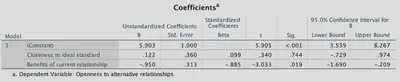
The b-values tell us about the relationship between openness to alternative relationships and each predictor. For the variable Ideal, the b-value is positive (b = 0.122), indicating a positive relationship between Ideal and Alternatives. However, this predictor is not significant, t(8) = 0.34, p = 0.74, because the associated p-value is very much larger than 0.05. This variable, therefore, doesn’t help Celia much with convincing Zach he should consider an alternative relationship to Alice - especially as Celia seems to be very close to what Zach might consider his ideal woman (same taste in music, etc.).
For the variable Benefit, the b-value is negative ($ b = −0.950 $), indicating a negative relationship between Benefit and Alternatives, i.e., the more benefits you see in your current relationship the less likely you are to search for alternatives. This predictor is a significant predictor of openness to alternative relationships, t(8) = −3.033, p = 0.02. Celia could argue that since Alice had vanished without any warning, belittles him constantly, is obsessed with science, isn’t interested in his music anymore, and Zach has implied that he and Alice had been drifting apart, that there are not currently many benefits in his relationship with Alice. That being so, based on this model, he should be more open to alternative relationships such as with Celia.
Puzzle 9
Write out the model in Puzzle 8. What value of Alternatives would you expect if someone had scored 6 on the variable Ideal, and 7 on Benefit?
$$ \begin{aligned} \hat{Y}_i &= \hat{b}_0 + \hat{b}_1X1_i + \hat{b}_2X2_i \\ \hat{\text{Alternatives}}_i &= \hat{b}_0 + \hat{b}_1\text{Ideal}_i + \hat{b}_2\text{Benefit}_i\\ &= 5.90 + 0.12\text{Ideal}_i - 0.95\text{Benefit}_i \end{aligned} $$
If someone had a score of 6 on Ideal and 7 on Benefit, then we can plug these values into the model and find that you’d expect to get a value of
$$ \begin{aligned} \hat{\text{Alternatives}}_i &= 5.90 + 0.12\text{Ideal}_i - 0.95\text{Benefit}_i \\ &= 5.90 + (0.12 \times 6) + (-0.95 \times 7)\\ &= -0.03. \end{aligned} $$
This predicted value illustrates the fact that models are approximations of reality. A value is $ −0.03 $ is ridiculous because the rating scale ranges from 0 to 10, so this score is impossible.
Puzzle 10
A Bayes factor version of the model in puzzle 8 is shown in Output 14.11 (in the book and reproduced below). What three models have been tested, and which one should we choose?
The output shows the Bayes factor when we include only Ideal as a predictor, only Rewards, or when we include both. Each model is compared to an ‘intercept only’ model; that is, a model with no predictors. All of the models have Bayes factors above 1 (although barely when only Ideal is included), but the largest Bayes factor is for when only Rewards is included as a predictor (the evidence for the model is 10.15 times that of the null). Ideal and Rewards together have a reasonable effect (the evidence for the model is 3.94 times that of the null), but the effect of Ideal alone produces a Bayes factor of only 1.02 (the evidence for the model is only 1.02 times that of the null). Therefore, we would favour model 2, in which Rewards is the only predictor.
Bayes factor analysis
--------------
[1] Ideal           : 1.018349 ±0.01%
[2] Rewards         : 10.15071 ±0%
[3] Ideal + Rewards : 3.939688 ±0%

Against denominator:
  Intercept only
---
Bayes factor type: BFlinearModel, JZS
Output 14.11 (reproduced)