Chapter 12
Assumptions
Puzzle 1
In Milton’s Meowsings 12.1 (in the book), Milton presents data from an experiment involving 10 people in which he measured the concentration of a chemical in his spray, and the level of oxytocin in the person whom he sprayed. Table 12.1 (in the book) shows these data. What is a residual? Compute the residuals for each participant in Table 12.1.
A residual is the difference between the value of the outcome predicted by the model and the value of the outcome actually observed. In equation form, a residual is defined as:
$$ \text{residual}_i= \text{observed}_i-\text{predicted}_i $$
This equation means that the residual (or error) for person i is their actual score on the outcome variable minus the score for the outcome predicted by the model. To calculate the residuals in Table 12.1 we would need to subtract the predicted level of oxytocin in each participant (predicted values) from the observed value for each participant (oxytocin). I have copied Table 12.1 from the book below, but added a new column at the end containing the residual for each participant.
| Reproduction of Table 12.1, but including an additional column containing the residual value for each participant | ||||
|---|---|---|---|---|
| ID | Oxytocin $Y_i$ |
Concentration $X_i$ |
Predicted value $\hat{Y}_i$ |
Residual $Y_i-\hat{Y}_i$ |
| 1 | 2.45 | 74 | 2.70 | -0.25 |
| 2 | 3.67 | 79 | 2.83 | 0.84 |
| 3 | 0.87 | 58 | 2.29 | -1.42 |
| 4 | 2.11 | 38 | 1.77 | 0.34 |
| 5 | 3.29 | 82 | 2.91 | 0.38 |
| 6 | 1.33 | 20 | 1.30 | 0.03 |
| 7 | 1.09 | 7 | 0.97 | 0.12 |
| 8 | 2.68 | 37 | 1.74 | 0.94 |
| 9 | 1.44 | 44 | 1.92 | -0.48 |
| 10 | 1.58 | 50 | 2.08 | -0.50 |
Puzzle 2
Describe what you understand by the term ‘linear model’.
The linear model is defined by an equation that describes a straight line which is very commonly used by scientists to describe the data they have collected:
$$ \text{outcome}_i=(\text{model})+\text{error}_i $$
$$ \text{outcome}_i= b_0 + b_1X_i + \epsilon_i $$
We can make the linear model more complicated by measuring a second predictor variable and including that in the model too, like in this equation:
$$ Y_i = b_0 + b_1X_{1i} + + b_2X_{2i} + \epsilon_i $$
In general, we can expand the model to include more and more predictors of the outcome:
$$ Y_i= b_0 + b_1X_{1i} + + b_2X_{2i} + \dots + b_nX_{ni} + \epsilon_i $$
All this means is that we can carry on adding predictor variables until we reach the nth one, that is, the last one that we want to include. All predictor variables have a parameter that quantifies the relationship between the predictor variable and the outcome, so bn is the parameter for the last predictor variable.
Puzzle 3
Describe the assumptions of additivity and linearity.
The assumptions of additivity and linearity are the most important ones because they mean that the real-world process that you want to model can, in reality, be described by your linear model. Linearity is the assumption that the outcome variable is, in reality, linearly related to any predictors (i.e., their relationship can be summed up by a straight line). Additivity is the assumption that if you have several predictors then their combined effect is best described by adding their effects together.
Puzzle 4
What is meant by the phrase ‘independent errors’?
The assumption of independent errors means that a given error in prediction from the model should not be related to and, therefore, affected by a different error in prediction. Violating the assumption of independence invalidates confidence intervals and significance tests of parameter estimates. The estimates themselves will be valid but not optimal if we use the method of least squares.
Puzzle 5
Describe with an example what is meant by homogeneity of variance. Describe the ways in which you can find out whether you have it in your data.
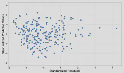
Let’s use the example from Chapter 12 in the book, in which a sample of people were either exposed to oxytocin or not before being asked to rate how much they trusted a stranger. In this experiment we have two groups: one group who were exposed to oxytocin and one group who were not. The assumption of homogeneity of variance is met if the variances in the two groups are roughly equal, and the spread of scores for trust is approximately the same at each level of the oxytocin variable (i.e., the spread of scores is very similar in the oxytocin and no-oxytocin groups). To find out whether you have homogeneity of variance in your data, you can look at a plot of the standardized predicted values from your model against the standardized residuals (zpred vs. zresid). If it has a funnel shape then the assumption has been violated. Additionally, when comparing groups, a significant Levene’s test (i.e., a p-value less than 0.05) reveals a problem with the assumption of homogeneity of variances; however, there are good reasons not to use this test (see Milton’s Meowsings 12.3 in the book). Finally, the variance ratio (Hartley’s Fmax) is the largest group variance divided by the smallest, and this value needs to be smaller than the published critical values – although people often use a value of 2 as a threshold, for no particularly good reason that I can find.
Puzzle 6
What is heteroscedasticity?
Heteroscedasticity is the opposite of homoscedasticity. This occurs when the residuals (errors) at each level of the predictor variable(s) have unequal variances. For example, the residuals might be tightly packed around the model at one end of the scale but widely spread around the model at the other end, giving rise to a characteristic funnel shape.
Puzzle 7
How does heteroscedasticity affect the linear model?
Heteroscedasticity will bias the confidence intervals and significance tests for the parameter estimates in your model. Confidence intervals can be ‘extremely inaccurate’ when homoscedasticity cannot be assumed.
Puzzle 8
What does Figure 12.10 (in the book) tell us about whether the assumption of homoscedasticity has been met for this model?
Figure 12.10 tells us that the assumption of homoscedasticity has been violated for this model. We can tell this because the residuals take the form of the characteristic funnel shape: they become less spread out across the graph.
Puzzle 9
What is the assumption of normality and what does it affect in the linear model?
This is the assumption that the sampling distribution or distribution of residuals is normal. Estimates of the model parameters (the bs) will be optimal using the method of least squares if the model residuals are normal. Confidence intervals and significance tests rely on the sampling distribution being normal, and we can assume this in large samples because of the central limit theorem. In small samples bootstrapping should be applied to get robust estimates of b.
Puzzle 10
The Kolmogorov–Smirnov test can be used to look at whether scores have a normal distribution. Why might we not want to use this test?
When samples are large and normality is less of a problem the K-S test will be overpowered and likely to be significant, leading you to believe that the data are non-normal in a situation where non-normality does not actually matter. Conversely, in small samples, where we might need to worry about normality, the K-S test will not have the power to detect it and so is likely to encourage us not to worry about something that we probably ought to. The same basic argument applies for homogeneity of variance tests.
Puzzle 11
What is multicollinearity and how do we look for it?
Multicollinearity occurs when there is a strong relationship between two or more predictors. The most extreme example would be perfect collinearity, which is when at least one predictor is a perfect linear combination of the others. In other words, they are perfectly related: as one variable increases, the other increases by a proportional amount. One simple method to look out for multicollinearity is to look at the correlation coefficients between predictors: if they are very high, such as values around 0.8 or more, then that is a reasonable indication that there might be a problem. You can also look at the variance inflation factor (VIF), which indicates whether a predictor has a strong linear relationship with the other predictor(s) in the model. If the largest VIF is greater than 10 then there is cause for concern, and if the average VIF is substantially greater than 1 then the model may be biased. You could also use the tolerance statistic, which is the reciprocal of the VIF (1/VIF): values below 0.1 indicate a serious problem and values below 0.2 suggest a potential problem.