Chapter 3
Summarizing data
Puzzle 1
Describe the following terms: frequency, relative frequency, proportion and percentage.
- Frequency is the number of times that a score, range of scores or category occurs.
- Relative frequency is the frequency of a score, range of scores or category expressed relative to the total number of observations:
$$ \text{relative frequency} = \frac{\text{frequency of response}}{\text{total number of responses}} = \frac{f}{N} $$
- Relative frequencies are proportions. A proportion in statistics usually quantifies the portion of all measured data in a particular category in a scale of measurement. In other words, it is the frequency of a particular score/category relative to the total number of scores:
$$ \text{proportion} = \frac{\text{frequency of score/category}}{\text{total number of observations}} = \frac{f}{N} $$
- We can convert a relative frequency or proportion to a percentage by multiplying it by 100
$$ \text{percentage} = \text{proportion} \times 100 = \frac{f}{N} \times 100 $$
Puzzle 2
Draw the frequency distribution of the RAS scores (with scores not grouped by class intervals).
Your hand drawn graph should look something like the one in Figure 1.
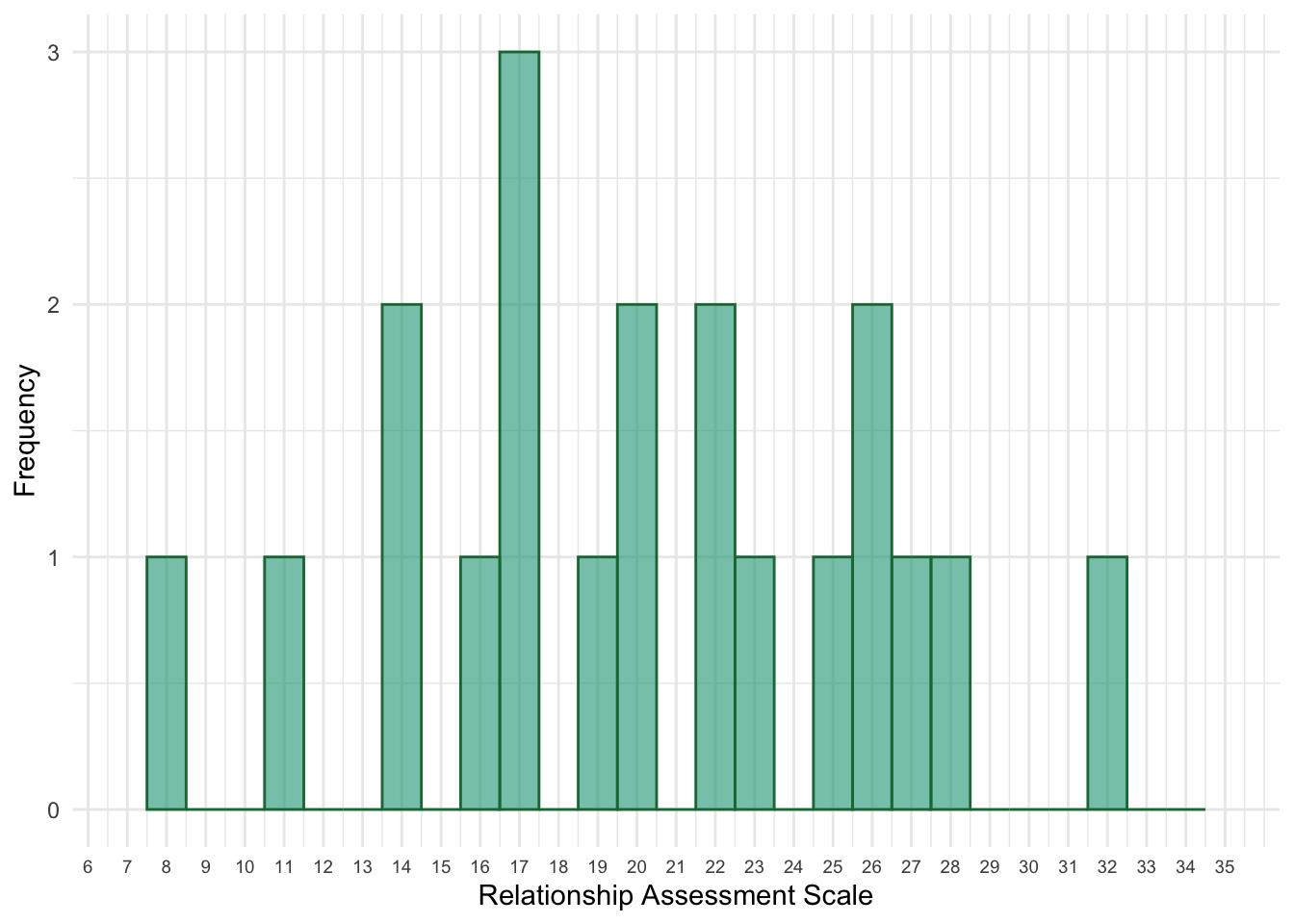
Figure 1: Histogram of RAS scores
Puzzle 3
In this chapter Zach looked at 20 women’s ratings of how important certain characteristics are in romantic partners. Here are the data for the characteristic wants to have children: 1, 1, 9, 1, 10, 3, 7, 6, 7, 2, 2, 9, 8, 2, 8, 6, 9, 2, 9, 6. Produce a frequency table of these data that includes: frequencies, relative frequencies, percentages, cumulative frequency, cumulative percentage
The answers to this puzzle can be found in Table 1.
| Rating | Frequency | Cumulative frequency | Relative frequency | Percentage | Cumulative percentage |
|---|---|---|---|---|---|
| 1 | 3 | 3 | 0.15 | 15% | 15% |
| 2 | 4 | 7 | 0.20 | 20% | 35% |
| 3 | 1 | 8 | 0.05 | 5% | 40% |
| 6 | 3 | 11 | 0.15 | 15% | 55% |
| 7 | 2 | 13 | 0.10 | 10% | 65% |
| 8 | 2 | 15 | 0.10 | 10% | 75% |
| 9 | 4 | 19 | 0.20 | 20% | 95% |
| 10 | 1 | 20 | 0.05 | 5% | 100% |
Puzzle 4
For the data in the previous question, remembering that scores of 0–5 mean ‘unimportant’ and 6–10 mean ‘important’, what percentage of adolescent women in this sample thought that it was important that their partners wanted to have children in the future?
The largest observed score below 6 (i.e. in the unimportant category) in the data was 3. If we look at the cumulative percentage column in Table 1, we can see that the cumulative percentage of the response of 3 was 40%. Therefore, 40% of the sample gave a rating in the ‘unimportant’ category, which means that 60% gave a rating of 6 or more (i.e. in the ‘important’ category). Therefore, 60% of adolescent women (in this sample) thought that it was important that their partners wanted to have children in the future.
Puzzle 5
Zach was worried that he was unappealing to women because he dropped out of college. Here are the ratings of the 20 women in the chapter for the characteristic finished education: 9, 8, 5, 4, 7, 3, 10, 7, 6, 4, 4, 8, 9, 1, 7, 3, 7, 6, 10, 9. Draw a histogram of these data. Do you think most of these women think that it is important that their relationship partner finished their college education?
Your hand-drawn histogram should look like Figure 2. Looking at the histogram, we can see that the scores are spread out across the whole scale, there is no accumulation of scores at either end of the scale. This indicates that the characteristic finished education wasn’t consistently rated as either important or unimportant – views were quite varied.
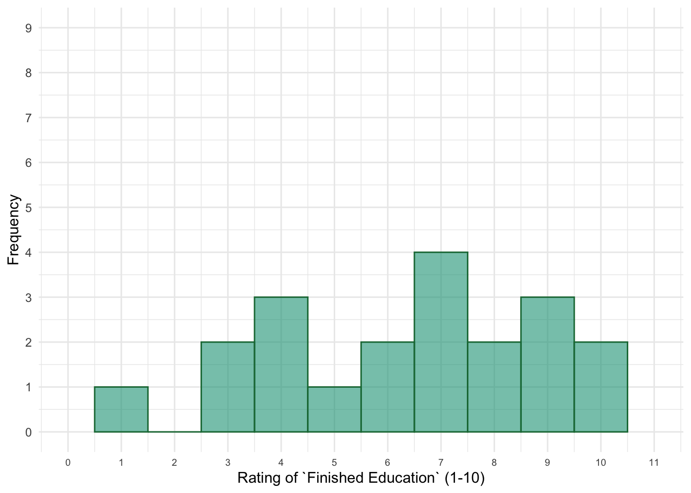
Figure 2: Histogram of 20 women’s ratings of the importance of a relationship partner having finished their education
Puzzle 6
The polygon in Figure 3.10 (in the book and reproduced below) shows the ratings for the characteristic romantic. From this image reconstruct the raw data.
Looking at the polygon, we can see that no one gave a rating of 0, 1, 2 or 6. One person gave a rating of 3, one gave a 4 and one a 5. Eight people gave a rating of 7, four people gave a rating of 8, two people gave a rating of 9 and three people gave a rating of 10. Therefore, the raw data for the 20 women are:
3, 4, 5, 7, 7, 7, 7, 7, 7, 7, 7, 8, 8, 8, 8, 9, 9, 10, 10, 10.
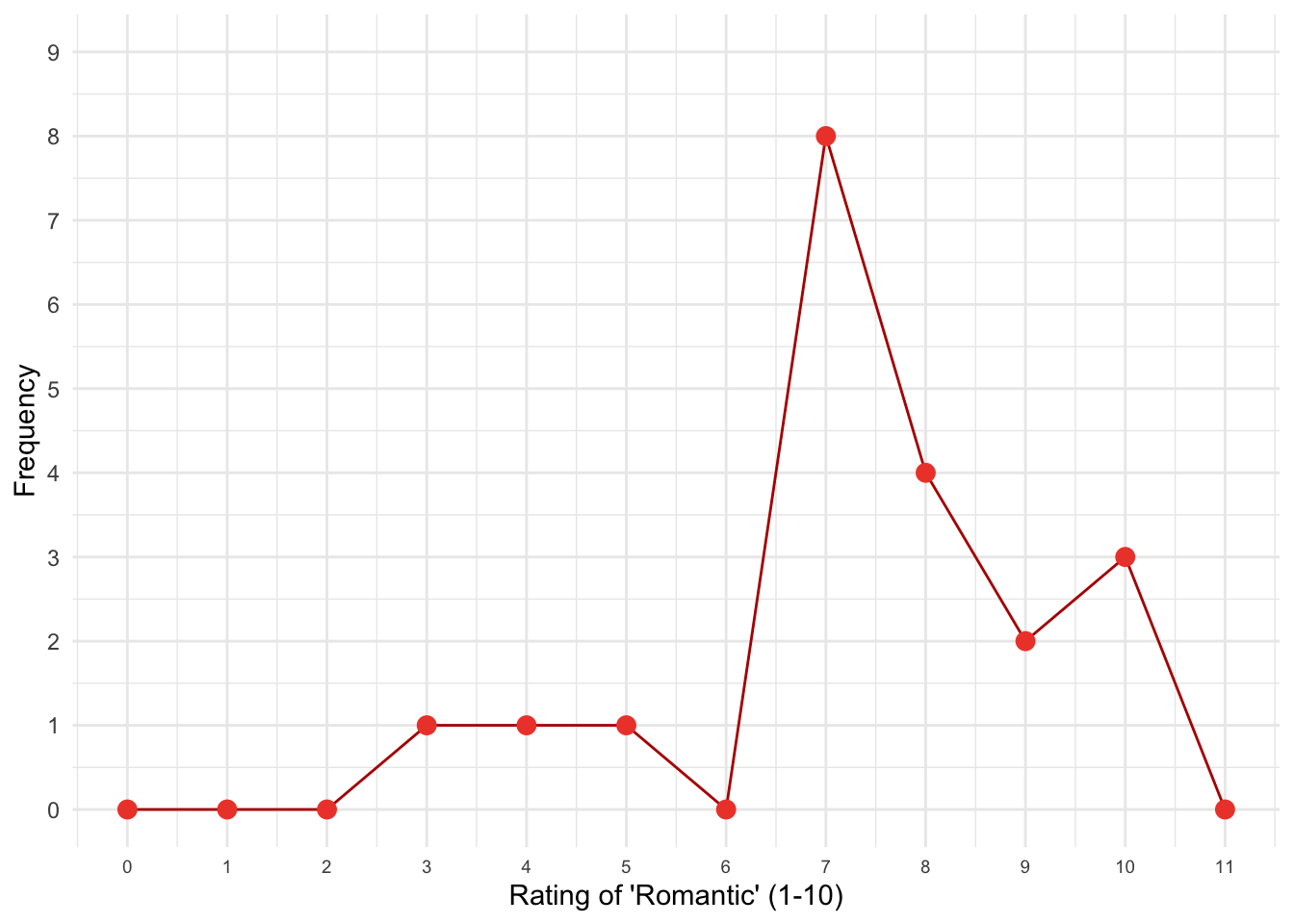
Figure 3: Figure 3.10 (reproduced): Polygon of the ratings for the characteristic 'romantic'
Puzzle 7
Here are the ratings for the same 20 women for the characteristic attractive appearance: 4, 10, 9, 8, 7, 8, 10, 8, 7, 3, 9, 10, 8, 10, 7, 9, 9, 9, 8, 7. Draw a frequency distribution of these scores.
Your hand-drawn frequency distribution should look like Figure 4.
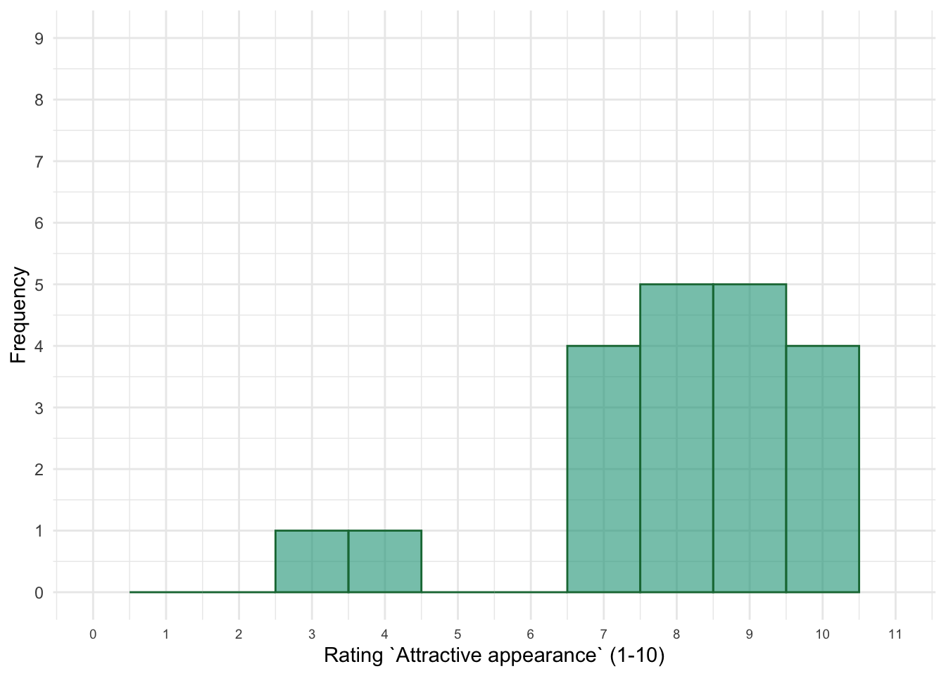
Figure 4: Histogram of ratings of the importance of an attractive appearance in a relationship partner
Puzzle 8
Here are the ratings for the same 20 women for the characteristic creativity: 7, 6, 5, 4, 5, 8, 9, 5, 5, 7, 4, 5, 5, 10, 7, 3, 5, 9, 1, 7. Draw a frequency polygon of these scores.
Your hand-drawn frequency polygon should look like Figure 5.
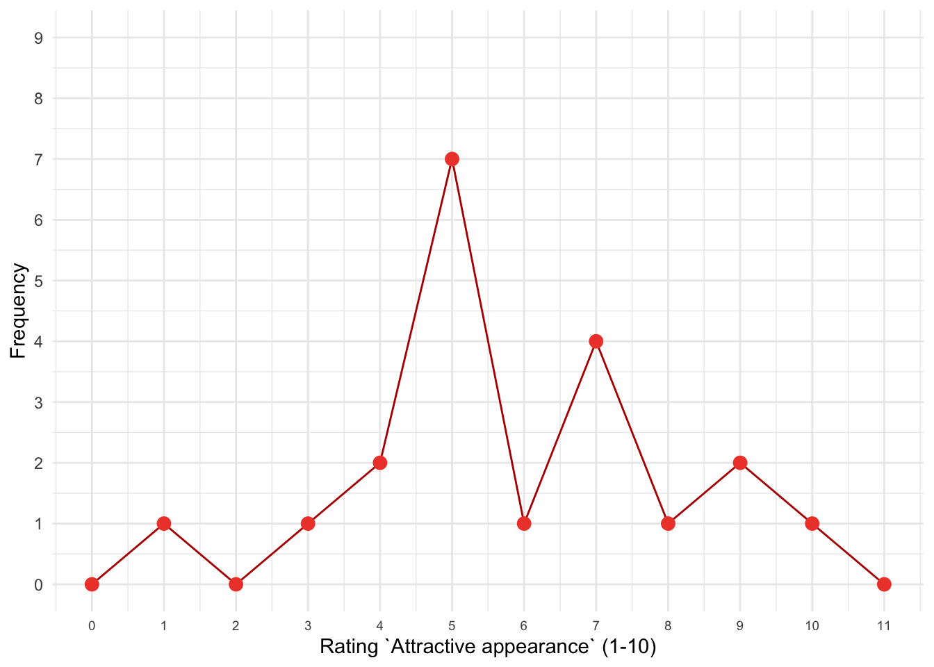
Figure 5: Frequency polygon of ratings of the importance of creativity in a relationship partner
Puzzle 9
The histogram in Figure 3.11 (in the book and reproduced below) shows the ratings for the characteristic honesty. From this image reconstruct the raw data.
Looking at the histogram (Figure 6), we can see that no-one gave ratings of 1, 2, 3, 4, 5, 6 or 7 because there are no bars above 0 for any of these ratings. Four people gave a rating of 8, four gave a rating of 9 and twelve gave a rating of 10. Therefore, the raw data for the 20 women are:
8, 8, 8, 8, 9, 9, 9, 9, 10, 10, 10, 10, 10, 10, 10, 10, 10, 10, 10, 10.
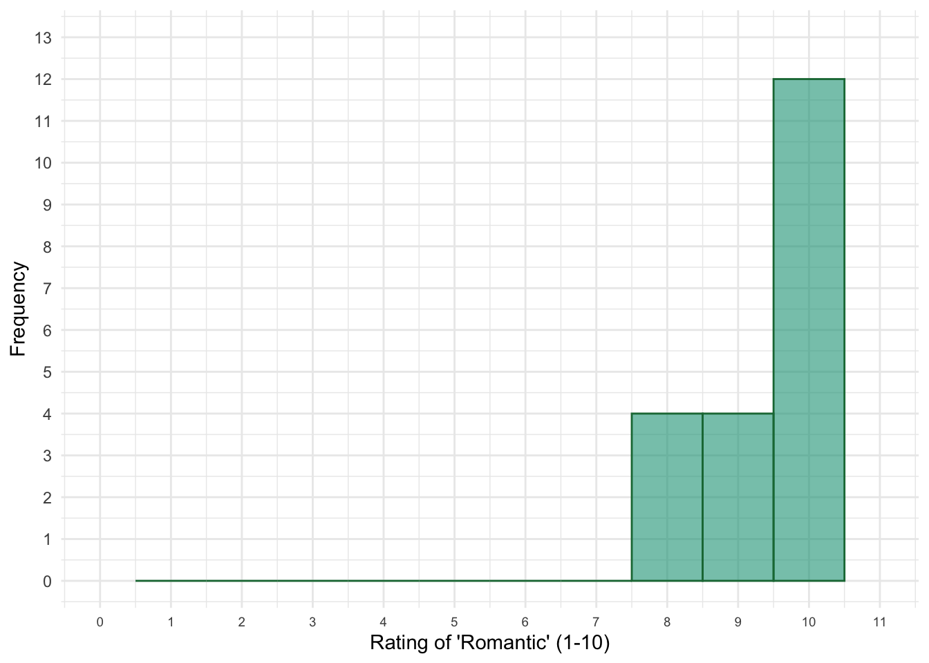
Figure 6: Figure 3.11 (reproduced): Histogram of the ratings for the characteristic 'honesty'
Puzzle 10
Based on the histograms and polygons for the previous three Puzzles, what characteristic do the women in the sample most consistently find important in a romantic partner: attractive appearance, creativity or honesty? Explain your answer.
Looking back at the three plots (Figures 3-6) we can see that honesty is the characteristic that is consistently important in a romantic partner. We know this because the bars on the graph are clustered at the high end of the scale, honesty was always rated between 8 and 10, and over half of the sample gave it a rating of 10. Attractive appearance also received mostly high ratings of between 7 and 10 but the ratings are more evenly spread over this range than for the honesty characteristic. The ratings for creativity, on the other hand, were more spread out across the whole scale. The highest number of ratings occurred around the middle of the scale, suggesting that there wasn’t consistent agreement on the importance of this characteristic in a romantic partner: most of the women rated it as neither important nor unimportant.
Puzzle 11
Sketch the shape of a normal distribution.
Your graph should look like Figure 7.
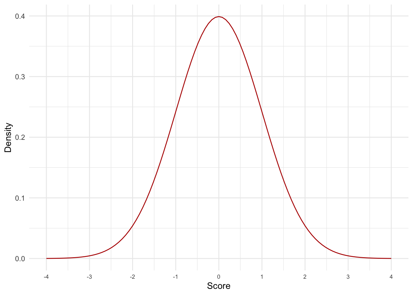
Figure 7: A normal distribution (the curve shows the idealized shape)
Puzzle 12
Look at the histograms in Figure 3.1 (in the book and reproduced below). For each one comment on:
How symmetrical you think they are
The graphs for high salary and ambitious both look fairly symmetrical. The graph for humour is less symmetrical and the graph for kind is not symmetrical at all.
How flat or pointy they are
The histogram for high salary is very flat: the bars are of quite similar heights across all of the categories. In fact, each point along the scale was endorsed by a similar number of people, which suggests that there is no consistent pattern valuing a high salary as an important characteristic in this sample.
The histogram for kind is very pointy at the high end of the distribution. This suggests that most women rated kindness as an important characteristic in a romantic partner. The histograms for humour and ambitious are not particularly pointy or flat, although the one for humour certainly has a heavy tail at the top end of the scale (i.e., more scores than you might expect). It is interesting that the vast majority of women put their response above 5, which means they thought these characteristics were important to some extent.
How skewed they are, and whether the skew is positive or negative
The histogram for high salary isn’t very skewed at all; the scores are evenly spread out across the whole scale, giving a very flat distribution. The histogram for kind, on the other hand, is highly negatively skewed; we can tell this because the frequent scores are clustered at the higher end and the tail points towards the lower, or more negative, scores. The histogram for humour shows a slight negative skew. The histogram for ambitious isn’t particularly skewed but, if anything, it shows slight positive skew.
These patterns indicate that kindness was consistently rated as a highly important characteristic in a romantic partner, as was humour. Ambition was also consistently rated as an important characteristic, but to a lesser extent than kindness and humour. However, there was no consistent pattern for the characteristic high salary: about as many women in the sample rated this characteristic as highly important as rated it as unimportant.
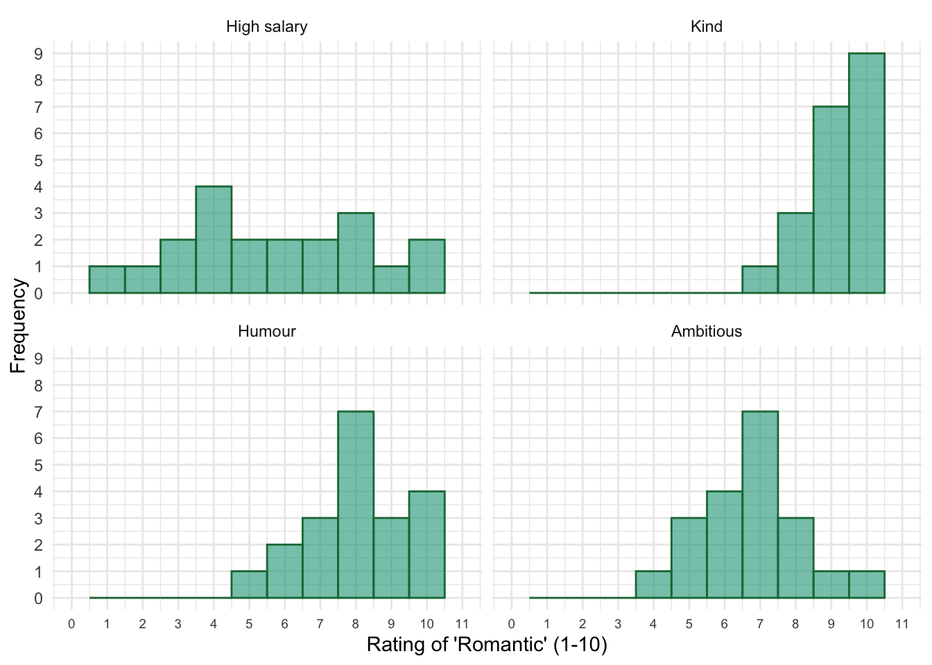
Figure 8: Figure 3.1 (reproduced): Histograms of the importance of four characteristics in their partners